📐 Visualizing Quantum Confinement with Brillouin Zone Analysis

Giovanni Gravili October 15, 2024 Mathematica, Physics, Quantum Mechanics

Quantum confinement fundamentally changes how electrons behave. Take a bulk semiconductor and squeeze it down to a quantum well, then to a quantum wire, and finally to a quantum dot, and you’ll watch the smooth density of states transform into discrete energy levels. This progression from continuous bands to atomic-like spectra isn’t just theoretical, it’s the physics behind everything from LEDs to quantum computers. For a solid-state physics course project, I built a complete band structure calculator in Mathematica that visualizes this transformation by computing Brillouin zones, plotting band structures along high-symmetry paths, and calculating density of states for systems confined in 0, 1, 2, and 3 dimensions. The project revealed how reciprocal space geometry directly determines electronic properties, and how Voronoi tessellations, purely mathematical constructs, map perfectly onto physical Brillouin zones. Mathematica’s symbolic and geometric capabilities made it natural to work with these abstractions, turning graduate-level solid-state physics into interactive visualizations I could manipulate and explore.

The challenge of understanding electronic band structure begins with reciprocal space. While real space describes where atoms sit in a crystal, reciprocal space (or k-space) describes the allowed momentum states for electrons. The first Brillouin zone (1BZ) is the fundamental domain in k-space, analogous to a unit cell in real space. For a body-centered cubic (bcc) lattice, the 1BZ has a characteristic truncated octahedral shape. By calculating energy eigenvalues along high-symmetry paths through this zone and sampling the full volume, we can understand how quantum confinement affects electronic structure.

My whole collection of Mathematica Notebook files is available at this link.

Constructing the Brillouin Zone

The foundation is the reciprocal lattice. For a bcc crystal with real-space basis vectors, the reciprocal lattice is face-centered cubic (fcc). I define the basis for the reciprocal lattice:

basis = {{1, -1, 1}, {1, 1, -1}, {-1, 1, 1}}

These vectors generate the reciprocal lattice points (G-vectors) through integer linear combinations. To construct the first Brillouin zone, I generate all reciprocal lattice points within a reasonable range and compute the Voronoi tessellation:

gvecs = Tuples[Range[-7, 7], 3].basis
vmesh = VoronoiMesh[gvecs]

The Voronoi cell centered at the origin is the first Brillouin zone. This construction has a beautiful geometric interpretation: the 1BZ consists of all points in k-space closer to the origin than to any other reciprocal lattice point. The Voronoi tessellation automatically finds this region by constructing perpendicular bisecting planes between the origin and neighboring G-points.

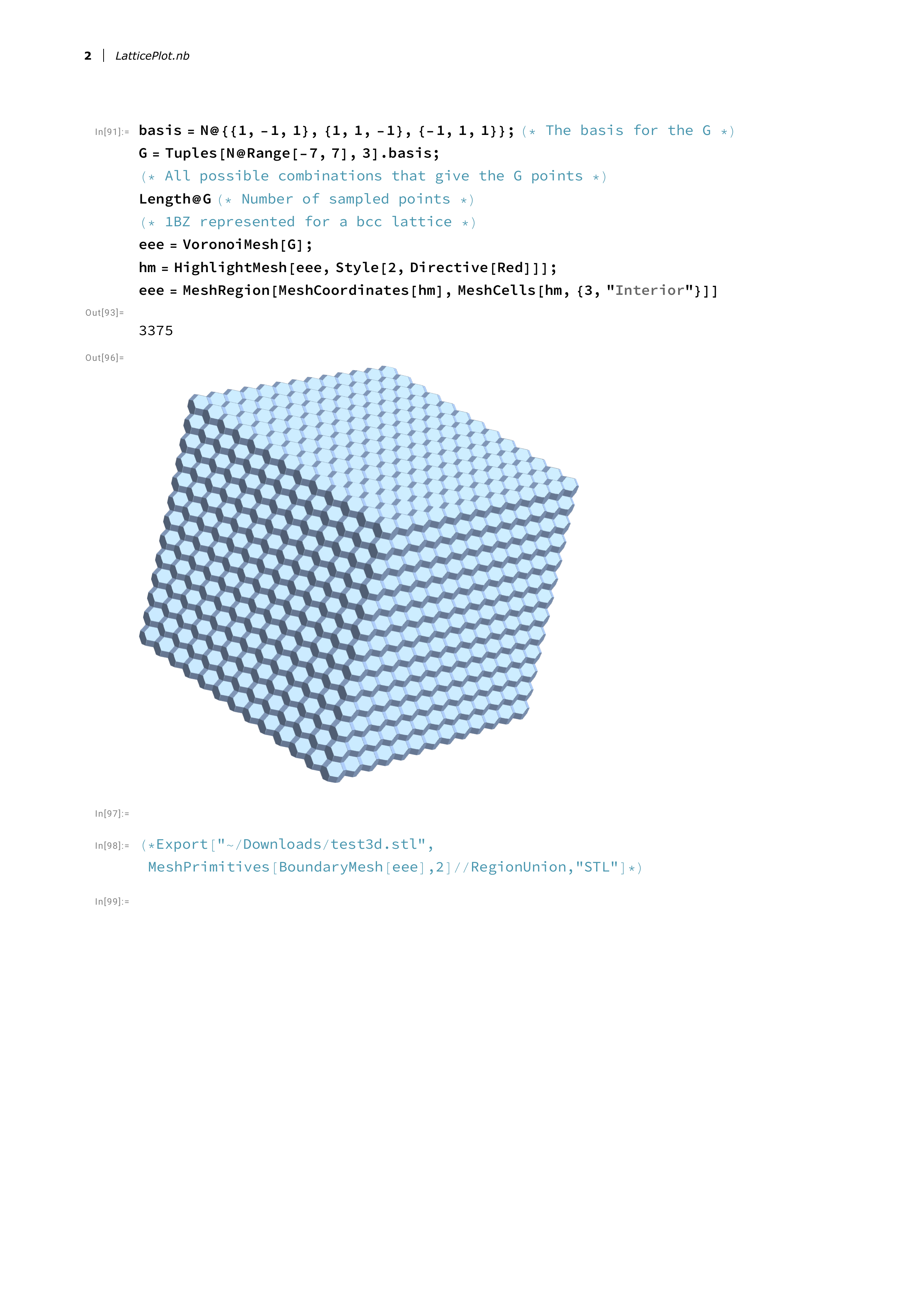
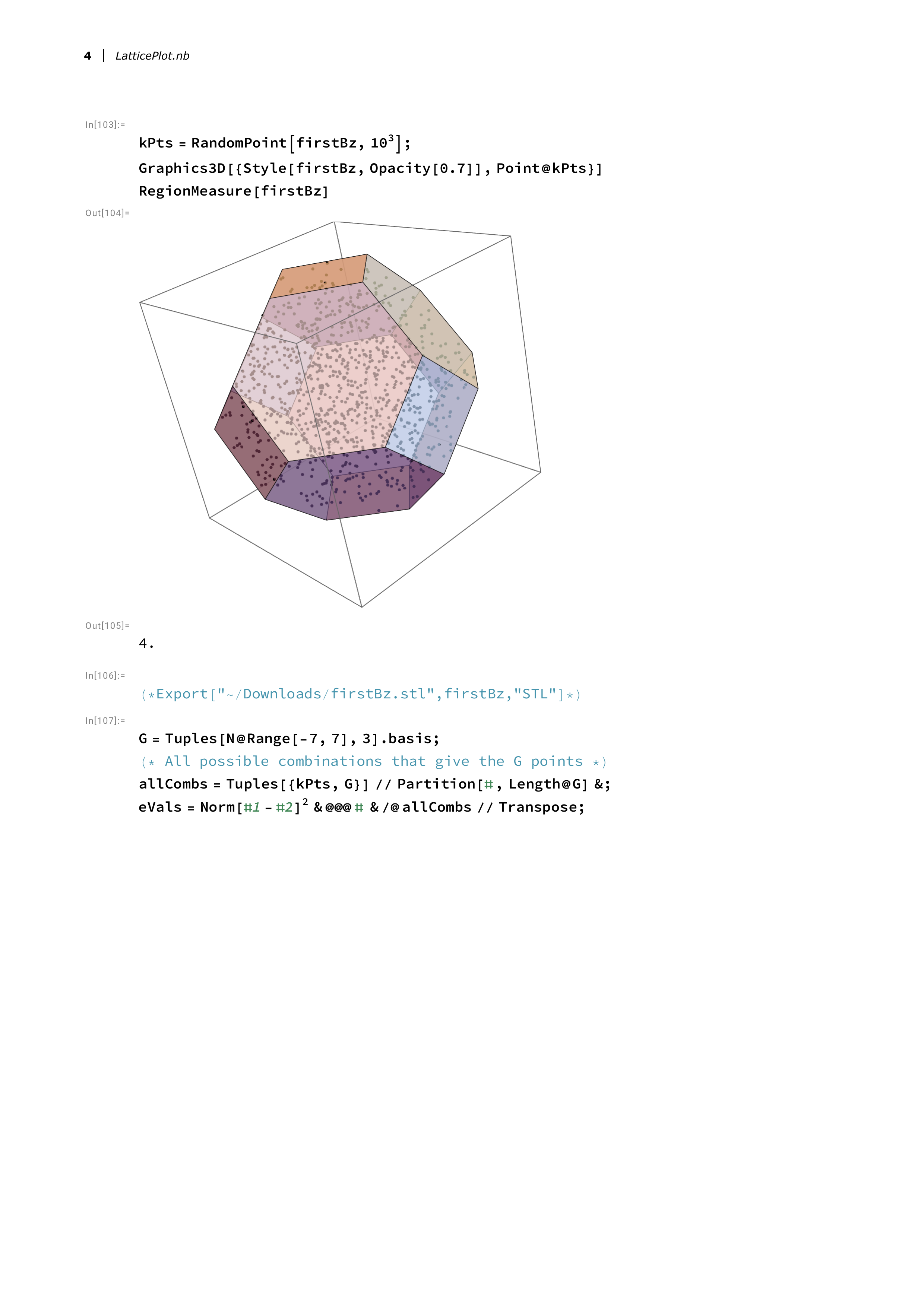
The resulting 3D mesh shows the characteristic shape of the bcc Brillouin zone. The mesh contains 3375 reciprocal lattice points, and the Voronoi construction identifies the interior region that forms the 1BZ. The volume of this zone is exactly 4 cubic units in reciprocal space, which can be verified with RegionMeasure[firstBz].

Band Structure Along High-Symmetry Paths

Electronic band structure is traditionally plotted along paths connecting high-symmetry points in the Brillouin zone. These points have special labels rooted in group theory: $\Gamma$ is the zone center, $X$ , $W$ , $L$ , $K$ , and $U$ are points on zone faces, edges, and corners. The conventional path for bcc crystals follows:

$L \to K \to U \to W \to \Gamma \to X \to W \to L \to \Gamma \to K \to U \to X$

This path can be broken into segments:

$L \to K \to U \to W \to \Gamma$ (outer boundary sweep)
$\Gamma \to X \to W \to L \to \Gamma$ (inner loop)
$\Gamma \to K \to U \to X$ (connecting high-symmetry edges)

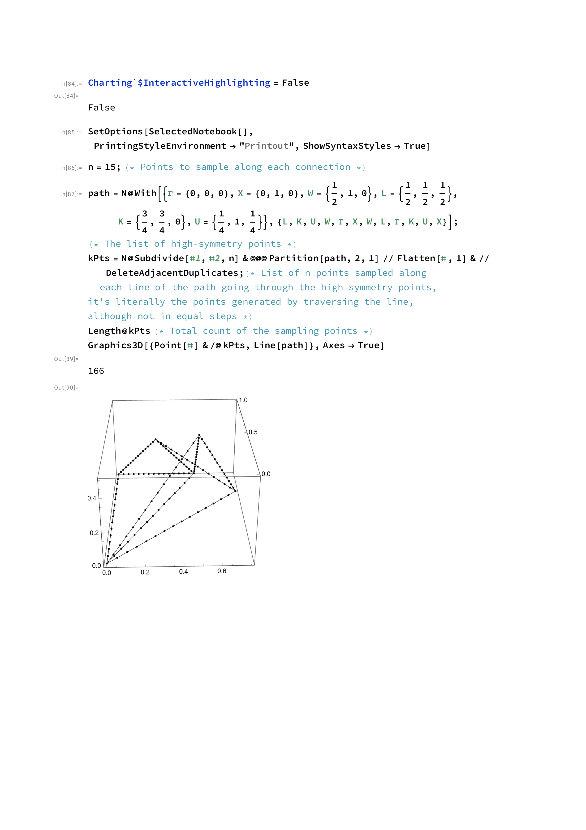
I define these points in fractional coordinates:

path = {
  Γ = {0, 0, 0},
  X = {0, 1, 0},
  W = {1/2, 1, 0},
  L = {1/2, 1/2, 1/2},
  K = {3/4, 3/4, 0},
  U = {1/4, 1, 1/4}
}

To compute the band structure, I sample 15 points along each segment of the path and calculate energy eigenvalues at each k-point. For a simple nearest-neighbor tight-binding model, the energy dispersion is:

$E(\mathbf{k}) = \sum_{\mathbf{G}} |\mathbf{k} - \mathbf{G}|^2$

This is essentially a free-electron model with periodic boundary conditions imposed by the reciprocal lattice. The implementation computes the distance from each k-point to all G-vectors and uses the squared norm as the energy:

kpts = Subdivide[#1, #2, n] & @@@ Partition[path, 2, 1] //
       Flatten[#, 1] & // DeleteAdjacentDuplicates

enrgs = With[{pairs = Tuples[{kpts, gvecs}] // Partition[#, Length@gvecs] &},
  Norm[#1 - #2]^2 & @@@ # & /@ pairs // Transpose
]

The calculation generates all k-point and G-vector pairs, computes the energy for each pairing, and transposes the result to group energies by k-point. This gives us multiple energy bands (each corresponding to a different G-vector) as functions of position along the path.

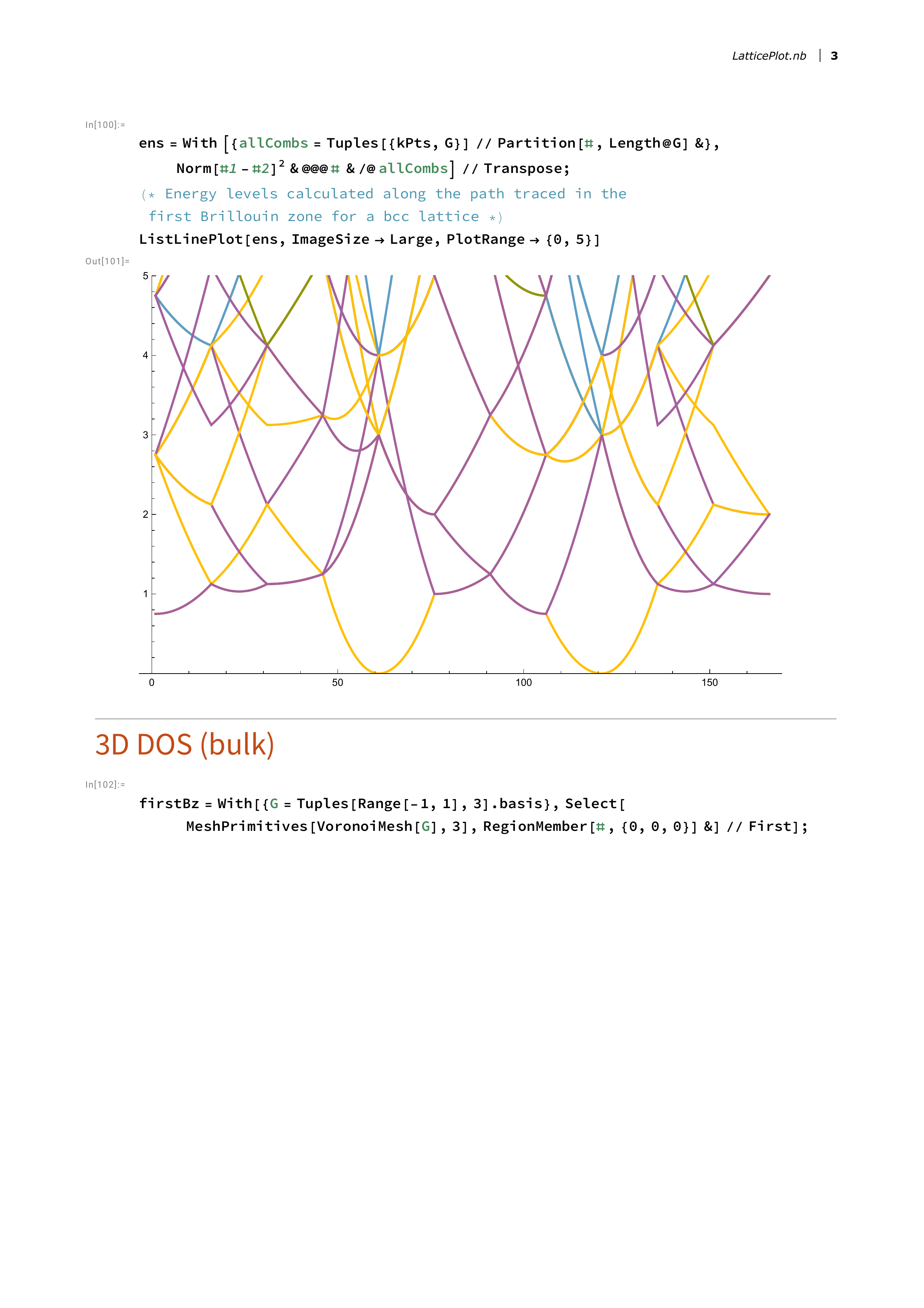
The band structure shows the characteristic features of a periodic potential. Bands cross and form avoided crossings, reflecting the symmetry of the underlying lattice. Energy gaps appear where bands do not overlap, corresponding to forbidden energy ranges. The colorful lines each represent a different band, and the horizontal axis traces the path through k-space from $L$ to $K$ to $U$ to $W$ to $\Gamma$ and so on.

Density of States in Three Dimensions

The density of states (DOS) tells us how many electronic states exist at each energy level. Rather than plotting energy as a function of k, we ask: for a given energy $E$ , how many k-points have that energy? To compute this, I sample the Brillouin zone uniformly with random points:

kpts = RandomPoint[firstBz, 10^3]

For each sampled k-point, I compute the energy eigenvalues using the same free-electron dispersion. The DOS is then the histogram of these energies:

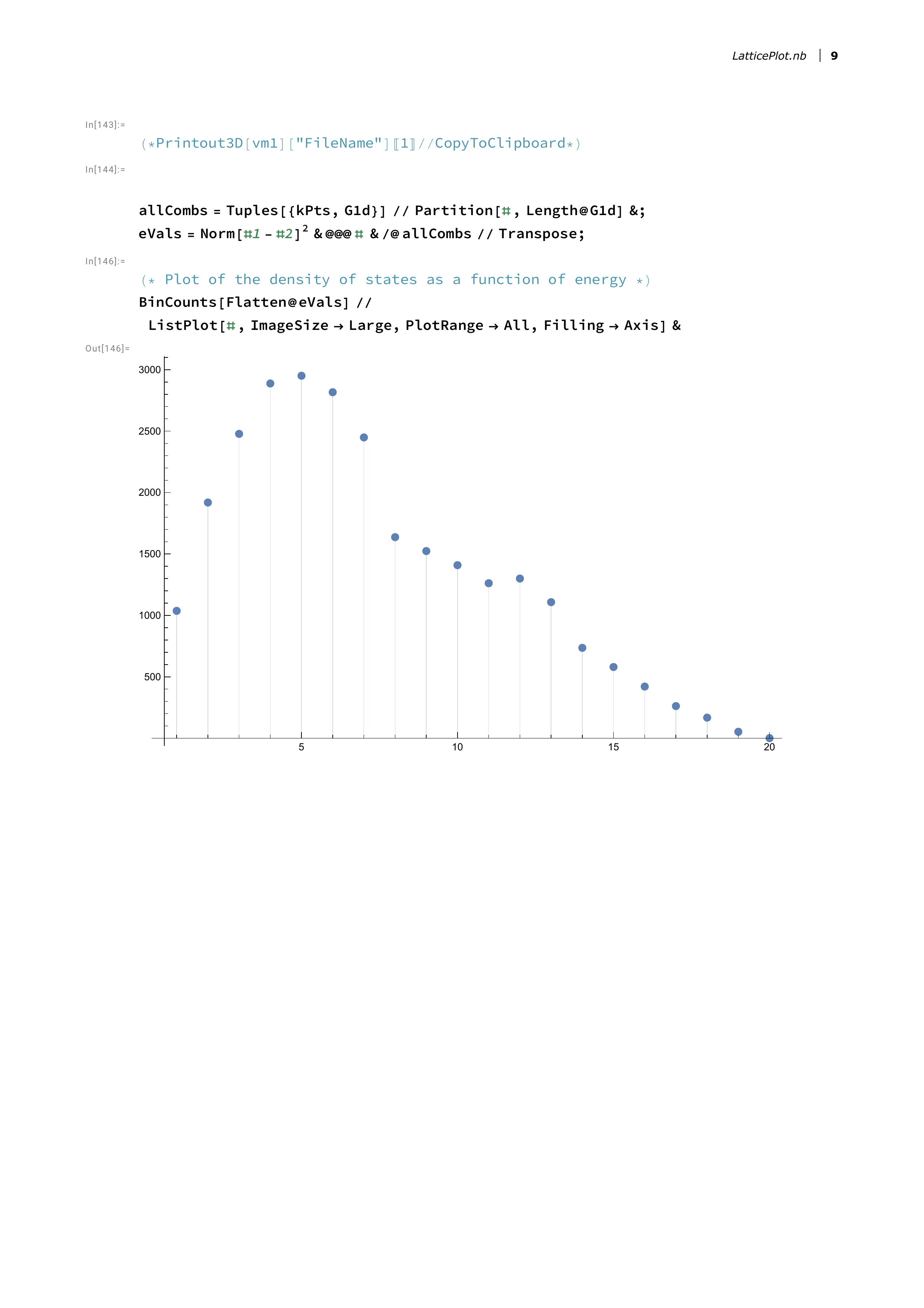
BinCounts[Flatten@enrgs] //
  ListLinePlot[#, ImageSize -> Large, Filling -> Axis, PlotRange -> All] &

The three-dimensional DOS for a free-electron gas follows the well-known $\sqrt{E}$ dependence at low energies. This characteristic shape emerges from the density of k-states in a sphere of radius $k = \sqrt{2mE}/\hbar$ combined with the parabolic dispersion relation.

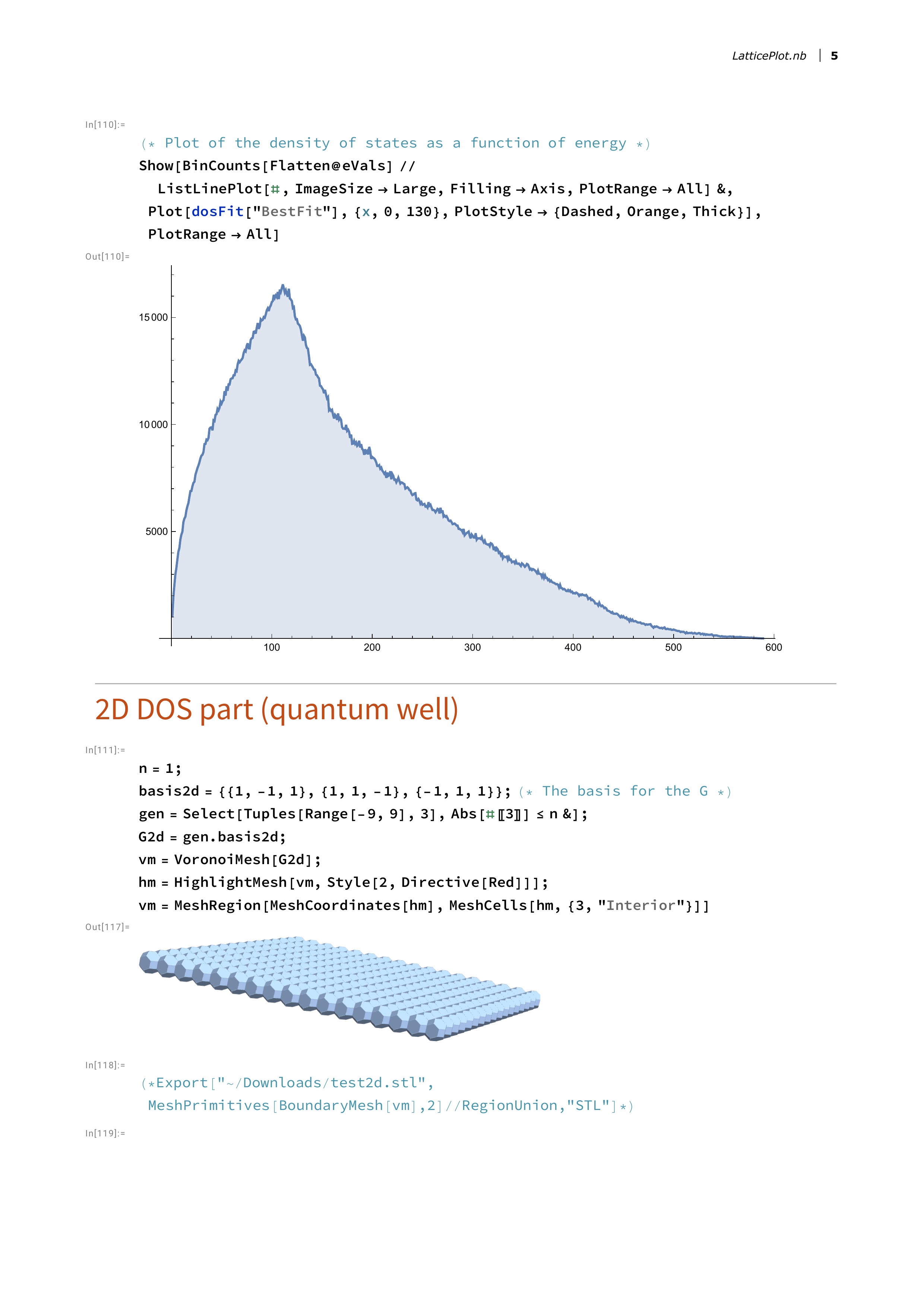
The smooth curve with $\sqrt{E}$ behavior is clearly visible. At higher energies, deviations appear due to the finite size of the Brillouin zone and the discreteness of the reciprocal lattice. The peak near energy 100 and the subsequent decay reflect the band structure features we saw earlier.

Quantum Confinement: From 3D to 2D

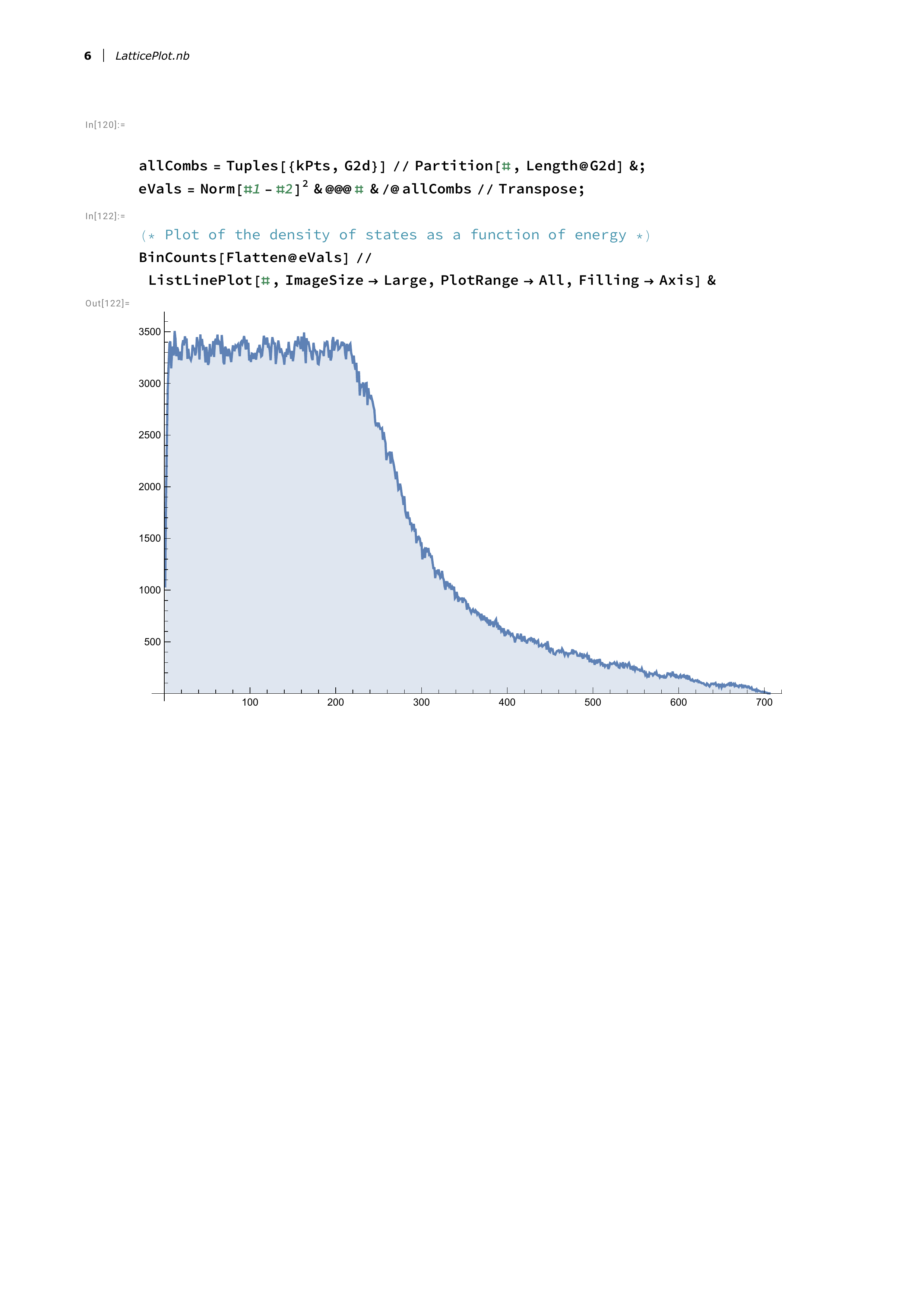
The power of this framework becomes apparent when we introduce quantum confinement. A quantum well confines electrons in one direction while allowing free motion in the other two. In k-space, this corresponds to restricting the reciprocal lattice to a slab. I implement this by filtering G-vectors:

gidx = Select[Tuples[Range[-9, 9], 3], Abs[#[[3]]] <= n &]
gv2d = gidx.basis2d

The parameter n = 1 limits the third component of the reciprocal lattice vectors, creating a confined system. The Voronoi mesh now forms a slab geometry. The structure is clearly two-dimensional: extended in the xy-plane but confined in z. This is the reciprocal space representation of a quantum well. The energy calculation proceeds identically, but now with the reduced set of G-vectors:

pairs = Tuples[{kpts, gv2d}] // Partition[#, Length@gv2d] &
enrgs = Norm[#1 - #2]^2 & @@@ # & /@ pairs // Transpose

The resulting density of states is fundamentally different:

The 2D DOS shows a plateau region at low energies rather than the $\sqrt{E}$ growth. This is the hallmark of two-dimensional systems: the density of states becomes constant, $\rho(E) \propto \text{constant}$ , because the area of a circle in k-space grows as $k \sim \sqrt{E}$ but the density of k-states per unit area is constant. The step-like features reflect the quantized subbands in the confined direction.

One-Dimensional Quantum Wires

Continuing the confinement progression, a quantum wire restricts motion to a single dimension. In reciprocal space, this means selecting G-vectors that satisfy:

gidx = Select[Tuples[Range[-14, 14], 3],
  #[[3]] <= n && #[[3]] >= -n && #[[2]] <= n && #[[2]] >= -n &]
gv1d = gidx.basis1d

Both the second and third components are restricted, leaving only variation along one axis. The Voronoi mesh becomes a one-dimensional chain:

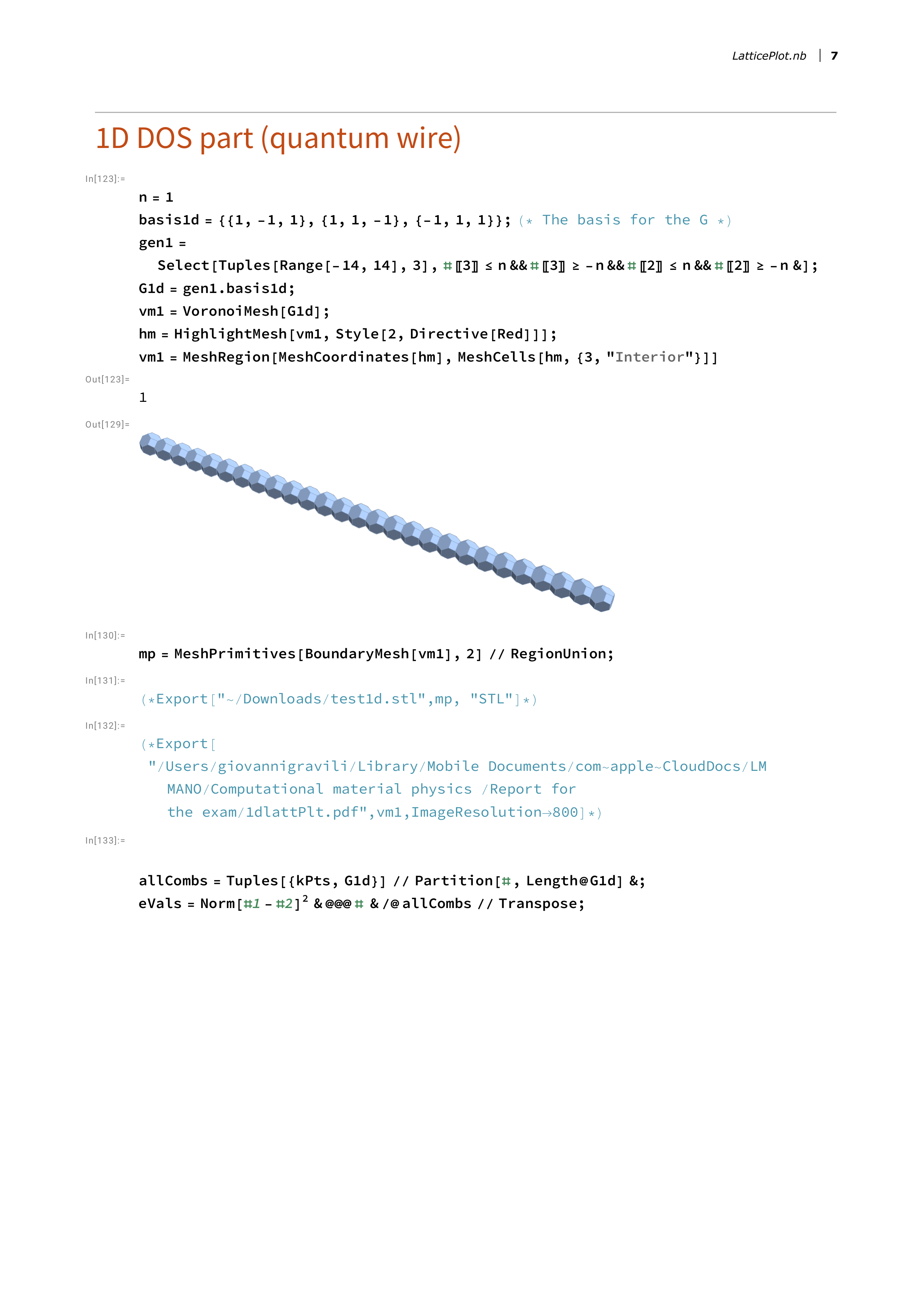
This elongated structure represents the allowed k-states in a quantum wire. Electrons can move freely along the wire axis but are confined in the perpendicular directions. The density of states for this system shows another dramatic change:

The 1D DOS exhibits sharp peaks and a characteristic $1/\sqrt{E}$ divergence at subband edges. This Van Hove singularity is a fundamental feature of one-dimensional systems: as energy approaches the bottom of a subband, the density of states diverges because $dE/dk \to 0$ at band extrema. The physical consequence is that electrons pile up at these energies, leading to strong optical absorption and other pronounced quantum effects.

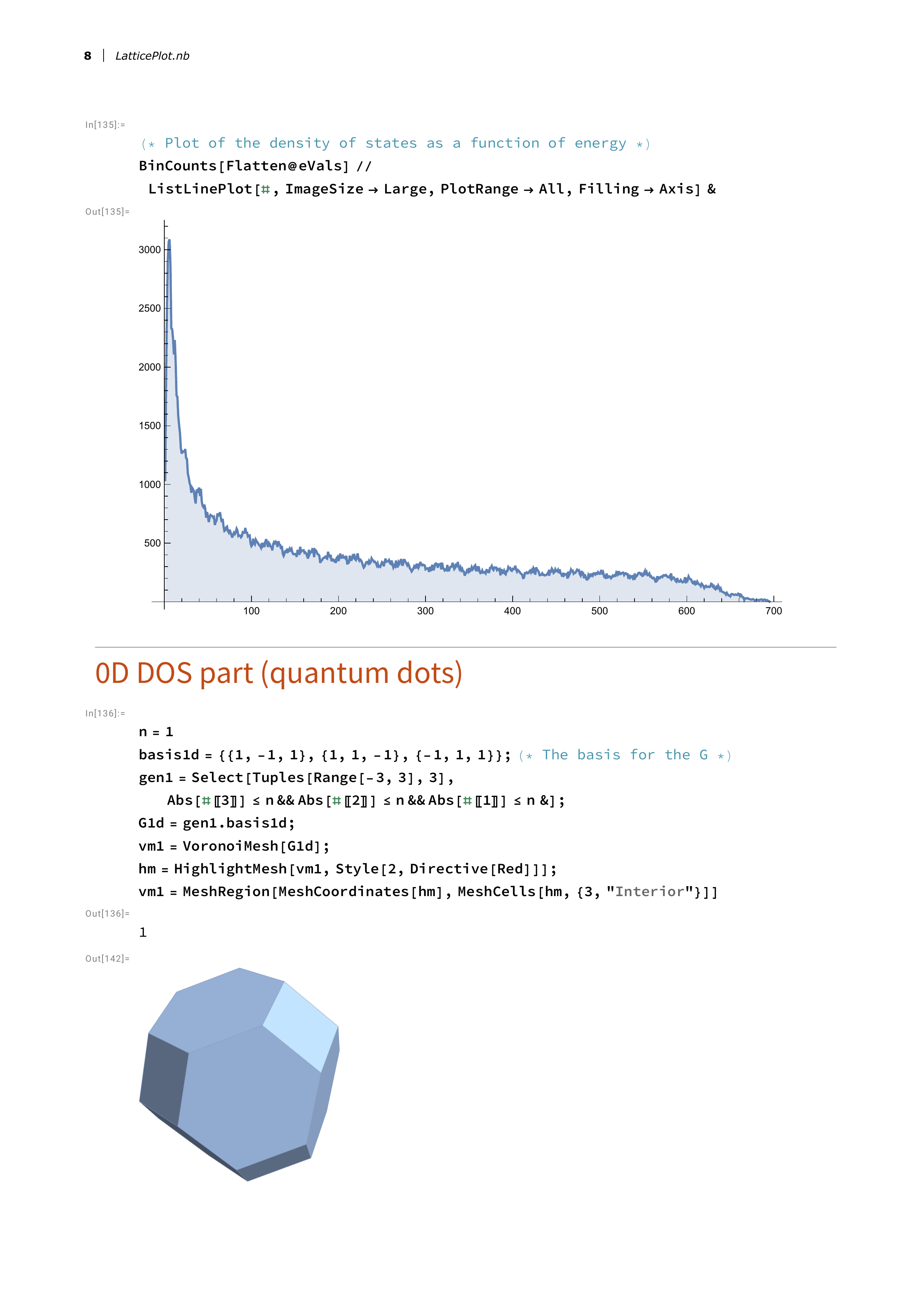
Zero-Dimensional Quantum Dots

The ultimate limit of confinement is a quantum dot: electrons confined in all three dimensions. This corresponds to selecting only a small region of reciprocal space:

gidx = Select[Tuples[Range[-3, 3], 3],
  Abs[#[[3]]] <= n && Abs[#[[2]]] <= n && Abs[#[[1]]] <= n &]
gv0d = gidx.basis0d

With n = 1, this selects only the nearest G-vectors, creating a discrete set of points. The Voronoi mesh becomes a single compact region. This finite polyhedron represents the entire allowed k-space for a quantum dot. There is no continuous dispersion relation, only discrete energy levels. The density of states becomes a series of delta functions:

The discrete spikes are the signature of zero-dimensional confinement. Each spike corresponds to a discrete energy eigenstate. There are no bands, no continuous dispersion, just a ladder of quantized levels like an artificial atom. This is why quantum dots are sometimes called “artificial atoms”: their electronic structure is fully discrete.

The Physics of Confinement

The progression from 3D to 2D to 1D to 0D reveals a fundamental principle: reducing dimensionality discretizes the density of states. The mathematical reason is clear from our construction. In three dimensions, we integrate over a continuous Brillouin zone volume, giving a smooth DOS. Confining one dimension quantizes momentum in that direction, turning an integral into a sum over discrete quantum numbers. Each additional confined dimension removes another integral, until in zero dimensions we are left with purely discrete states.

The physical consequences are profound. In bulk semiconductors (3D), electrons and holes form a continuum of states with smooth band edges. In quantum wells (2D), the DOS plateaus create enhanced exciton binding and improved laser efficiency. In quantum wires (1D), the Van Hove singularities lead to extremely strong light-matter coupling. In quantum dots (0D), the discrete spectrum enables single-photon sources and qubits.

The energy scale of these effects depends on the confinement length. For a particle in a box of size $L$ , the quantum confinement energy is:

$E_n \sim \frac{\hbar^2 \pi^2 n^2}{2m L^2}$

Smaller confinement (smaller $L$ ) pushes energy levels higher and increases their spacing. Modern nanofabrication can create quantum wells with $L$ of tens of nanometers, quantum wires with $L$ of a few nanometers, and quantum dots with $L$ below 10 nm. At these scales, confinement energies reach tens to hundreds of meV, well above thermal energy at room temperature.

Implementation and Visualization

One of the most satisfying aspects of this project was seeing the mathematical abstraction of reciprocal space become concrete through visualization. Mathematica’s VoronoiMesh function handles the geometric construction of Brillouin zones elegantly. The function takes a set of points (the reciprocal lattice) and computes the tessellation automatically:

vmesh = VoronoiMesh[gvecs]
hmesh = HighlightMesh[vmesh, Style[2, Directive[Red]]]
bzone = MeshRegion[MeshCoordinates[hmesh], MeshCells[hmesh, {3, "Interior"}]]

This pipeline generates the mesh, highlights surfaces, and extracts the interior region (the 1BZ). The resulting mesh can be exported as STL files for 3D printing:

Export["firstBz.stl", firstBz, "STL"]

I generated STL files for the 3D, 2D, 1D, and 0D Brillouin zones, creating physical models of reciprocal space geometry. Holding a 3D-printed Brillouin zone reinforces the reality of k-space: it is not just a mathematical construction but a physical object with volume, symmetry, and structure.

The energy calculations use functional programming patterns natural to Mathematica. The key operation is computing distances from k-points to G-vectors:

pairs = Tuples[{kpts, gvecs}] // Partition[#, Length@gvecs] &
enrgs = Norm[#1 - #2]^2 & @@@ # & /@ pairs // Transpose

Tuples[{kpts, gvecs}] creates all pairs of k-points and G-vectors. Partition[#, Length@gvecs] & groups these into blocks (one block per k-point, containing all G-vectors). The pure function Norm[#1 - #2]^2 & computes the squared distance, applied to each pair with @@@ (Apply at level 1). The outer Map applies this to each k-point block, and Transpose reorganizes the result into bands. This compact expression replaces what would be nested loops in imperative languages.

The density of states calculation uses BinCounts to histogram the energies:

BinCounts[Flatten@enrgs] //
  ListLinePlot[#, ImageSize -> Large, Filling -> Axis, PlotRange -> All] &

Flatten@enrgs collects all energies into a single list. BinCounts automatically chooses bin sizes and counts how many energies fall in each bin. The result is piped to ListLinePlot for visualization. This functional composition makes the intent clear: flatten, count, plot.

Building this band structure and density of states calculator demonstrates how computational tools can make abstract quantum mechanics tangible. The Brillouin zone is no longer just a diagram in a textbook but a 3D object I can visualize, rotate, and even print. The density of states is not just a formula but a curve I can compute, plot, and understand through direct calculation.

The progression from bulk (3D) to quantum well (2D) to quantum wire (1D) to quantum dot (0D) illustrates a fundamental principle of quantum mechanics: confinement leads to discretization. Each additional confined dimension removes a degree of freedom, replacing continuous bands with discrete subbands, and smooth density of states with sharp peaks. This is the physics underlying modern semiconductor nanostructures used in lasers, LEDs, single-photon sources, and quantum computers.

Working through the implementation in Mathematica taught me to appreciate the elegance of reciprocal space. The Voronoi construction automatically finds the Brillouin zone. The high-symmetry points naturally organize the band structure. The sampling and histogramming directly compute the density of states. The mathematical framework and the physical phenomena align perfectly.

The code itself is remarkably concise: a few dozen lines to define lattice vectors, construct Voronoi meshes, sample k-points, compute energies, and plot results. This conciseness is possible because the abstractions match the physics. Reciprocal lattice vectors are just matrices. The Brillouin zone is just a Voronoi cell. Energy bands are just functions of k. Density of states is just a histogram. Good abstractions make hard problems simple.

Most importantly, this project reinforced that computational physics is not about replacing analytical understanding with numerical brute force. It is about using computation to explore, visualize, and gain intuition for systems too complex for closed-form solutions. The band structures and DOS curves I generated are not approximations but exact solutions (within the free-electron model). The visualizations are not illustrations but actual data. Computation extends analytical physics, revealing structure that equations alone cannot easily show.

👨🏻‍🔬 Connect With Me

Other Projects